Basic image processes

Histogram
Histogram equalization
Image filtering

Histogram

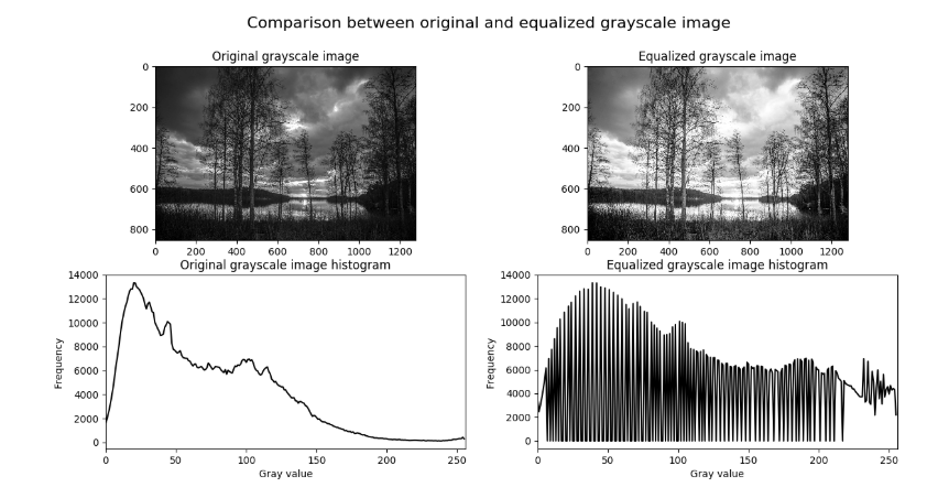
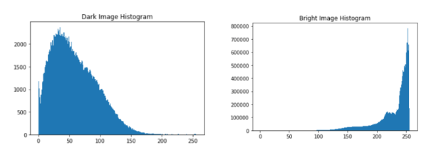
If the pixel brightness (gray level) in the image is regarded as a variable, its distribution is expressed as a gray histogram
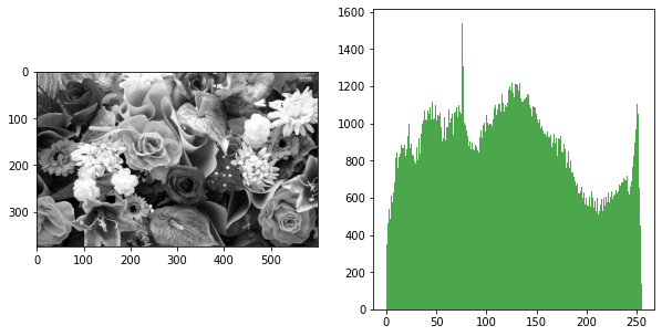
The grayscale histogram represents the number of pixels in the image that have a certain brightness range
The abscissa is the pixel brightness, and the ordinate is the frequency of the pixel brightness, which is the most basic statistical feature of the image

d_b_h

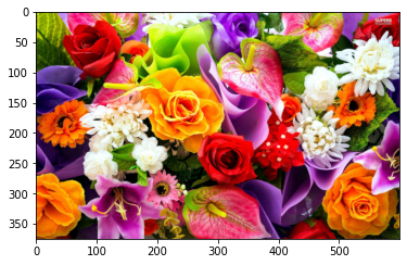
import cv2
from matplotlib import pyplot as plt
import numpy as np
import matplotlib.colors as mat_color

img_bgr = cv2.imread("./images/flowers_small.jpg")
img_rgb = cv2.cvtColor(img_bgr, cv2.COLOR_BGR2RGB)
print(img_rgb.shape)
no_norm = mat_color.Normalize(vmin=0, vmax=255, clip=False)
plt.imshow(img_rgb, norm=no_norm)
img_gray = cv2.imread("./images/flowers_small.jpg", flags=0)

(375, 600, 3)

png

plt.figure(figsize=(10, 5))
plt.subplot(1, 2, 1)
plt.imshow(img_gray, 'gray', norm=no_norm)
plt.subplot(1, 2, 2)
n, bins, patches = plt.hist(img_gray.ravel(), bins=256, color='green', alpha=0.7)

png

Histogram equalization

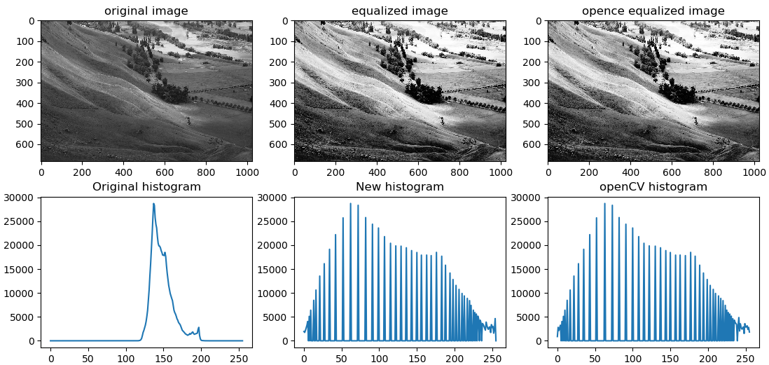
Histogram equalization is a technique for adjusting image intensities to enhance contrast
Let \(f\) be a given image represented as a \(M_{ray} \times M_{count}\) matrix of integer pixel intensities ranging from \(0\) to \(L − 1\). \(L\) is the number of possible intensity values, often \(256\). Let \(p\) denote the normalized histogram of \(f\) with a bin for each possible intensity. So

\[p_{n}=\frac{\text { number of pixels with intensity } n}{\text { total number of pixels }} \quad n=0,1, \ldots, L-1\]

The histogram equalized image \(g\) will be defined by

\[g_{i, j}=\operatorname{floor}\left((L-1) \sum_{n=0}^{f_{i, j}} p_{n}\right)\]

\(f_{i, j}\) represents the brightness of the pixel located at coordinate \((i, j)\)
floor() rounds down to the nearest integer
This is equivalent to transforming the pixel intensities, \(k\), of \(f\) by the function

\[T(k)=\operatorname{floor}\left((L-1) \sum_{n=0}^{k} p_{n}\right)\]

The motivation for this transformation comes from thinking of the intensities of \(f\) and \(g\) as continuous random variables \(X\), \(Y\) on \([0, L − 1]\) with \(Y\) defined by

\[Y=T(X)=(L-1) \int_{0}^{X} p_{X}(x) d x\]

\(p_X(x)\) is the probability density function of \(f\)
\(T\) is the cumulative distribution function of \(X\) multiplied by \((L − 1)\)
Assume for simplicity that \(T\) is differentiable and invertible
It can then be shown that \(Y\) defined by \(T(X)\) is uniformly distributed on \([0, L − 1]\), namely that \(\displaystyle p_Y(y) = \frac{1}{L - 1}\)

\[\begin{aligned} \int_{0}^{y} p_{Y}(z) d z &=\text { probability that } 0 \leq Y \leq y \\ &=\text { probability that } 0 \leq X \leq T^{-1}(y) \\ &=\int_{0}^{T^{-1}(y)} p_{X}(w) d w \end{aligned}\] \[\Rightarrow\quad\frac{d}{d y}\left(\int_{0}^{y} p_{Y}(z) d z\right)=p_{Y}(y)=p_{X}\left(T^{-1}(y)\right) \frac{d}{d y}\left(T^{-1}(y)\right)\]

Note that \(\displaystyle x = T^{-1}(y)\ \Rightarrow \ \frac{d}{d y} T(x)=\frac{d}{d y} T\left(T^{-1}(y)\right)=\frac{d}{d y} y=1\), so

\[\frac{d}{d y} T(x)=\frac{d}{d x}T(x)\cdot \frac{d x}{d y}=(L-1) p_{X}\left(x\right) \frac{d x}{d y}=(L-1) p_{X}\left(T^{-1}(y)\right) \frac{d}{d y}\left(T^{-1}(y)\right)=1\]

which means \(\displaystyle p_Y(y) = \frac{1}{L - 1}\)

hist_equa

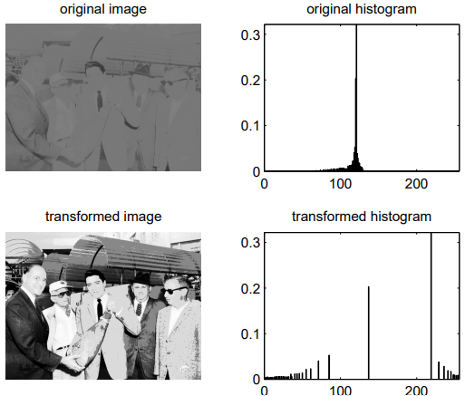
def compress_single(mean_value, img):
    # compress & flatten
    # allocate memory space and define compress rate
    hist = np.zeros(img.shape)
    for i in range(height):
        for j in range(width):
            rate = 0.875 + np.random.uniform(0, 0.05)
            hist[i][j] = mean_value * rate + img[i][j] * (1 - rate)
    return hist

height, width = img_gray.shape
mean_value = np.mean(img_gray)
print("mean value ->", mean_value)
img_hist = compress_single(mean_value, img_gray)
print("img_hist", np.min(img_hist), np.max(img_hist))
print("img_gray", np.min(img_gray), np.max(img_gray))
cv2.imwrite("./images/flowers_hist.jpg", img_hist)
print("compress done")

mean value -> 120.39762222222222
img_hist 105.34905636981311 137.2010426795889
img_gray 0 255
compress done

def show_hist_cdf(img):
    hist, bins = np.histogram(img.flatten(), 256, [0, 256])
    cdf = hist.cumsum()
    cdf_normalized = cdf * float(hist.max()) / cdf.max()
    plt.figure(figsize=(10, 7))
    plt.subplot(2, 2, 1)
    plt.imshow(img, 'gray', norm=no_norm)
    plt.subplot(2, 2, 2)
    plt.plot(cdf_normalized, color = 'b', linewidth=1.5)
    plt.hist(img.flatten(), 256, [0, 256], color='r', alpha=0.7)
    plt.legend(('cdf','histogram'), loc = 'upper left')
    plt.show()

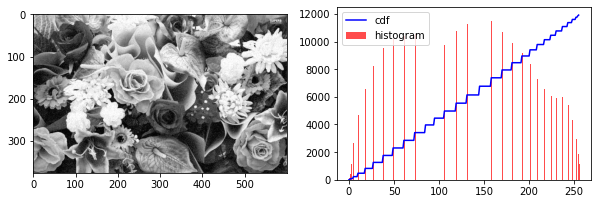
print("this is a good distributed image")
show_hist_cdf(img_gray)

this is a good distributed image

png

print("this is a compressed image, not good")
show_hist_cdf(img_hist)

this is a compressed image, not good

png

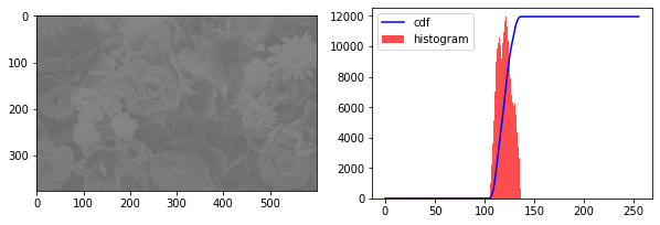
print("trsnafer the bad image to a good one")
img_hist = cv2.imread("./images/flowers_hist.jpg", flags=0)

img_equa = cv2.equalizeHist(img_hist)

cv2.imwrite("./images/flowers_equa.jpg", img_equa)
show_hist_cdf(img_equa) # after equalization
show_hist_cdf(img_hist)

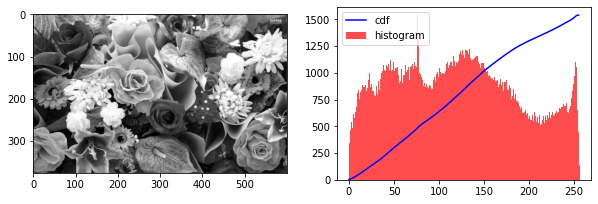
trsnafer the bad image to a good one

png

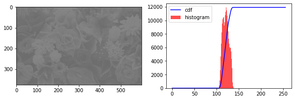
show_hist_cdf(img_equa) # after equalization
show_hist_cdf(img_gray)

png

print("now let's apply it in RGB images")
img_bgr = cv2.imread("./images/flowers_small.jpg")
img_rgb = cv2.cvtColor(img_bgr, cv2.COLOR_BGR2RGB)
R, G, B = cv2.split(img_rgb)

R_hist = compress_single(np.mean(R), R)
G_hist = compress_single(np.mean(G), G)
B_hist = compress_single(np.mean(B), B)

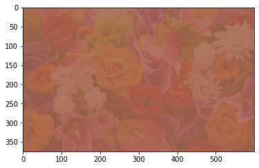
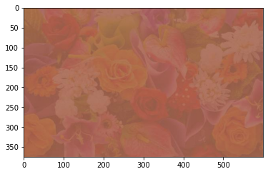
img_hist = cv2.merge((R_hist, G_hist, B_hist))
plt.imshow(img_hist.astype('uint8'), norm=no_norm)
# cv2.imwrite("./images/flowers_hist_rgb.jpg", img_hist.astype('uint8'))
plt.imsave("./images/flowers_hist_rgb.jpg", img_hist.astype('uint8'), 
           vmin=0, vmax=255)
print("compress RGB done")

now let's apply it in RGB images
compress RGB done

png

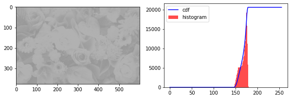
show_hist_cdf(R_hist)
show_hist_cdf(G_hist)
show_hist_cdf(B_hist)

png

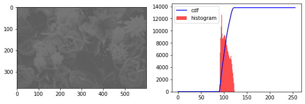
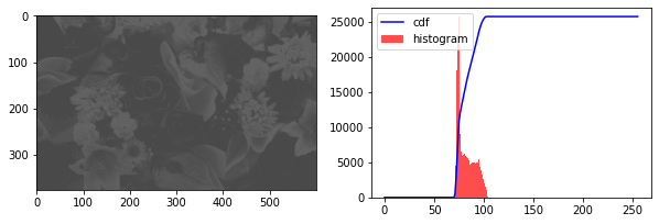
img_bgr = cv2.imread("./images/flowers_hist_rgb.jpg")
img_rgb = cv2.cvtColor(img_bgr, cv2.COLOR_BGR2RGB)
plt.imshow(img_rgb.astype('uint8'), norm=no_norm)

<matplotlib.image.AxesImage at 0x1696fa4dd30>

png

R, G, B = cv2.split(img_rgb)

R_equa = cv2.equalizeHist(R)
G_equa = cv2.equalizeHist(G)
B_equa = cv2.equalizeHist(B)

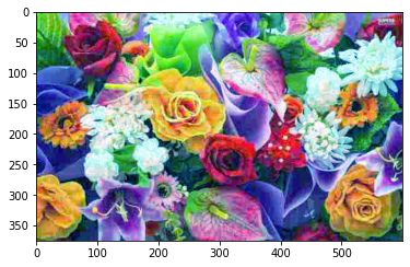
img_equa = cv2.merge((R_equa, G_equa, B_equa))
# cv2.imwrite("./images/flowers_equa_rgb.jpg", img_equa)
plt.imsave("./images/flowers_equa_rgb.jpg", img_equa, vmin=0, vmax=255)
plt.imshow(img_equa, norm=no_norm) # after equalization
print("compress RGB done")

compress RGB done

png

show_hist_cdf(R_equa) # after equalization
show_hist_cdf(G_equa)
show_hist_cdf(B_equa)

png

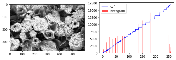
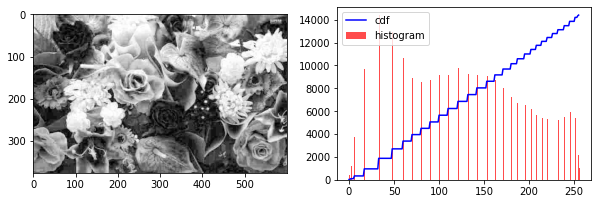
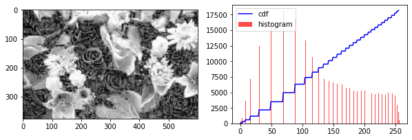
Image filtering

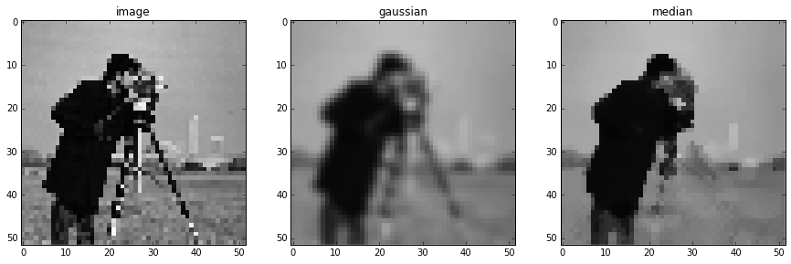
Image noise

Noise: factors that prevent people’s sense organs from comprehending the received source information
For example, a black and white image, whose brightness distribution is assumed to be \(f(x,y)\), then the brightness distribution \(R(x,y)\) that interferes with it is called image noise.
Image noise is unpredictable and can only be recognized by probability and statistical methods. It can be regarded as a multi-dimensional random process

Classification

Cause: External noise and internal noise
Whether the statistical properties change over time: stationary noise and non-stationary noise
Relationship between noise and signal: additive noise and multiplicative noise
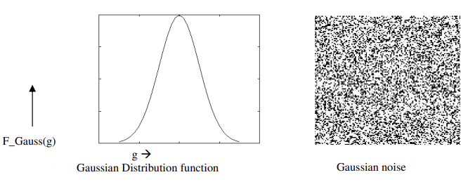
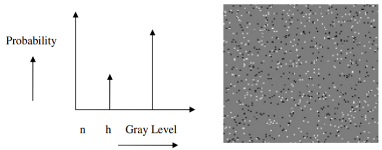
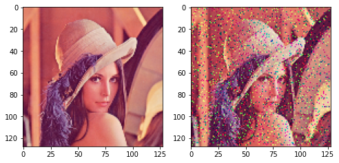
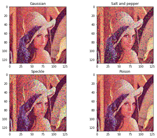
Specific types: Gaussian noise (probability distribution is Gaussian distribution) and Salt and pepper noise (random black and white dots), etc.

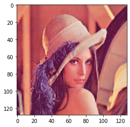
img_bgr = cv2.imread("./images/cv.png")
img_rgb = cv2.cvtColor(img_bgr, cv2.COLOR_BGR2RGB)
print(img_rgb.shape, img_rgb.size)
img_rgb = cv2.resize(img_rgb, (128, 128))
plt.imsave("./images/cv_small.png", img_rgb, vmin=0, vmax=255)
print(img_rgb.shape, img_rgb.size)
plt.imshow(img_rgb, norm=no_norm)

(512, 512, 3) 786432
(128, 128, 3) 49152

<matplotlib.image.AxesImage at 0x1696f9144c0>

png

Gaussian noise

gaussien

from PIL import Image

def gaussian_noise(image, sigma, gray=False, show=False, ret=True):
    # sigma: variance of gaussian noise
    if gray:
        noise = np.random.randn(image.shape[0], image.shape[1])
    else:
        noise = np.random.randn(image.shape[0], image.shape[1], image.shape[2])
    image = image.astype('int16')
    img_noise = image + noise * sigma
    img_noise = np.clip(img_noise, 0, 255)
    img_noise = img_noise.astype('uint8')
    if show:
        plt.figure(figsize=(12, 4))
        plt.subplot(1, 3, 1)
        plt.imshow(image, norm=no_norm)
        plt.subplot(1, 3, 2)
        plt.imshow(np.clip(noise * sigma, 0, 255).astype('uint8'), norm=no_norm)
        plt.subplot(1, 3, 3)
        plt.imshow(Image.fromarray(img_noise), norm=no_norm)
    if ret:
        return np.array(img_noise)
    else:
        return None

gaussian_noise(img_rgb, 70, show=True, ret=False)

png

Salt and pepper noise

salt_and_pepper

def salt_and_pepper(image, gray=False, show=False, ret=True):
    s_vs_p = 0.5
    amount = 0.07
    out = np.copy(image)
    # salt noise
    num_salt = np.ceil(amount * image.size * s_vs_p)
    coords = [np.random.randint(0, i - 1, int(num_salt))
              for i in image.shape]
    for i in range(len(coords[0])):
        if gray:
            out[coords[0][i]][coords[1][i]] = 255
        else:
            out[coords[0][i]][coords[1][i]][coords[2][i]] = 255
    # pepper noise
    num_pepper = np.ceil(amount* image.size * (1. - s_vs_p))
    coords = [np.random.randint(0, i - 1, int(num_pepper))
              for i in image.shape]
    for i in range(len(coords[0])):
        if gray:
            out[coords[0][i]][coords[1][i]] = 0
        else:
            out[coords[0][i]][coords[1][i]][coords[2][i]] = 0
    if show:
        plt.figure(figsize=(8, 4))
        plt.subplot(1, 2, 1)
        plt.imshow(image, norm=no_norm)
        plt.subplot(1, 2, 2)
        plt.imshow(out, norm=no_norm)
    if ret:
        return np.array(out)
    else:
        return None

salt_and_pepper(img_rgb, show=True, ret=False)

png

Speckle noise

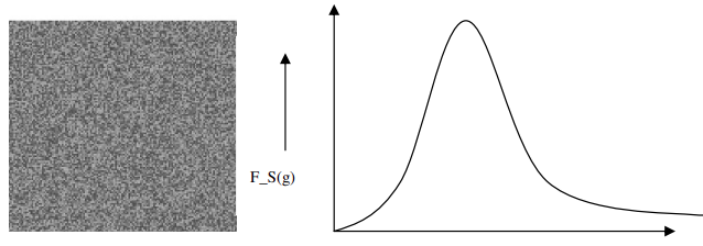
Multiplicative noise
In diagnostic examinations, this reduces image quality by giving images a backscattered wave appearance caused by many microscopic dispersed reflections flowing through internal organs
This makes it more difficult for the observer to distinguish fine details in the images

speckle

def speckle(image, sigma, gray=False, show=False, ret=True):
    # sigma: variance of gaussian noise
    if gray:
        noise = np.random.randn(image.shape[0], image.shape[1])
    else:
        noise = np.random.randn(image.shape[0], image.shape[1], image.shape[2])
    image = image.astype('int16')
    noise = noise * sigma
    img_noise = image + image * noise
    img_noise = np.clip(img_noise, 0, 255)
    img_noise = img_noise.astype('uint8')
    if show:
        plt.figure(figsize=(12, 4))
        plt.subplot(1, 3, 1)
        plt.imshow(image, norm=no_norm)
        plt.subplot(1, 3, 2)
        plt.imshow(np.clip(noise * 200, 0, 255).astype('uint8'), norm=no_norm)
        plt.subplot(1, 3, 3)
        plt.imshow(Image.fromarray(img_noise), norm=no_norm)
    if ret:
        return np.array(img_noise)
    else:
        return None

speckle(img_rgb, 0.35, show=True, ret=False)

png

Poison noise

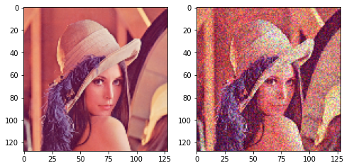
Poisson noise is produced by the image detectors’ and recorders’ nonlinear responses
This type of noise is determined by the image data. Because detecting and recording procedures incorporate arbitrary electron emission with a Poisson distribution and a mean response value, this expression is utilized

poisson

def poisson_noise(image, factor, show=False, ret=True):
    # factor: the bigger this value is, 
    # the more noisy is the poisson_noised image
    factor = 1 / factor
    image = image.astype('int16')
    img_noise = np.random.poisson(lam=image * factor) / float(factor)
    np.clip(img_noise, 0, 255, img_noise)
    img_noise = img_noise.astype('uint8')
    if show:
        plt.figure(figsize=(8, 4))
        plt.subplot(1, 2, 1)
        plt.imshow(image, norm=no_norm)
        plt.subplot(1, 2, 2)
        plt.imshow(img_noise, norm=no_norm)
    if ret:
        return np.array(img_noise)
    else:
        return None

poisson_noise(img_rgb, 7, show=True, ret=False)

png

How to prevent noise?

Image enhancement: Improve image intelligibility (Image filtering)
Image restoration: the improved image is as close to the original image as possible (Auto-encoder and Convolutional neural network)

def show_noisy(img_rgb):
    # salt_and_pepper is obviously different from each other
    # speckle is also obvious because it is a Multiplicative Noise
    # the other two is similar, their distributions are both convex function
    img_noisy = [gaussian_noise(img_rgb, 32), salt_and_pepper(img_rgb), 
                 speckle(img_rgb, 0.35), poisson_noise(img_rgb, 7)]
    titles = ["Gaussian", "Salt and pepper", "Speckle", "Poison"]
    plt.figure(figsize=(10, 8))
    for i in range(4):
        plt.subplot(2, 2, 1 + i)
        plt.imshow(img_noisy[i], norm=no_norm)
        plt.title(titles[i])
    return img_noisy

img_noisy_four = show_noisy(img_rgb)

png

Template operations and convolution operations

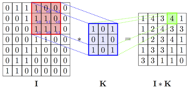
Image filtering, edge detection, etc. use template operations
Suppressing the noise of the target image under the condition of preserving the image details as much as possible is an indispensable operation in image preprocessing
The quality of the processing effect will directly affect the effectiveness and reliability of subsequent image processing and analysis
For example, a common smoothing algorithm is to average the value of a pixel in the original image and the values of 8 adjacent pixels around it, as the value of the pixel in the new image

\[\frac{1}{9}\left[\begin{array}{ccc}1 & 1 & 1 \\ 1 & 1^{*} & 1 \\ 1 & 1 & 1\end{array}\right]\]

Blur template

This is the BOX template, all the coefficients in the template have the same value, for \(5\times 5\) the BOX is

\[\frac{1}{25}\left[\begin{array}{ccccc} 1 & 1 & 1 & 1 & 1 \\ 1 & 1 & 1 & 1 & 1 \\ 1 & 1 & 1^{*} & 1 & 1 \\ 1 & 1 & 1 & 1 & 1 \\ 1 & 1 & 1 & 1 & 1 \end{array}\right]\]

Gaussian template

Template coefficients decrease as the distance from the template center increases
The size of the specific scale factor is determined by the 2D Gaussian function

\[H_{i, j}=\frac{1}{2 \pi \sigma^{2}} e^{-\frac{(i-k-1)^{2}+(j-k-1)^{2}}{2 \sigma^{2}}}\]

Where the \((2k+1)*(2k+1)\) is the size of template，\(i\) 、\(j\) represents the coordinate
For examplt, the \(3\times 3\) , \(\sigma = 0.3\) template is

\[\frac{1}{16}\left[\begin{array}{ccc} 1 & 2 & 1 \\ 2 & 4^{*} & 2 \\ 1 & 2 & 1 \end{array}\right]\]

Median filtering

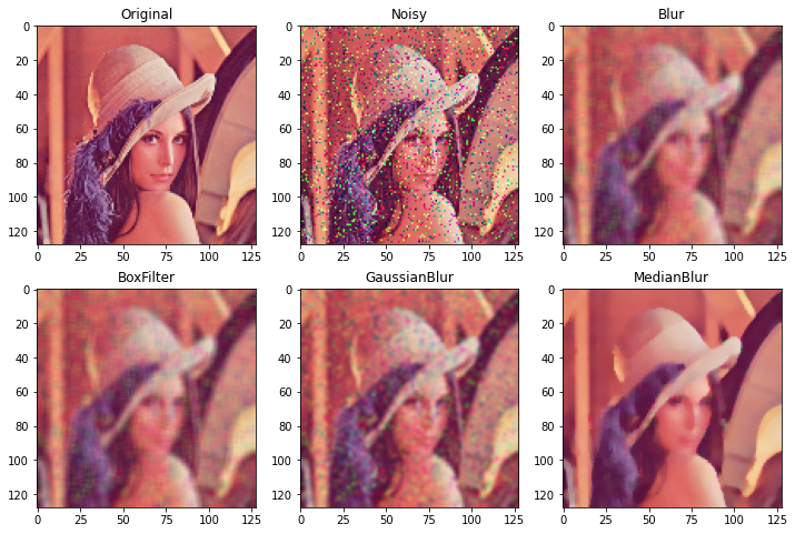
Median filtering is to use a moving window of odd points, and replace the value of the center point of the window with the median value of each point in the window
Assuming there are five points in the window with values \(80\), \(90\), \(200\), \(110\) and \(120\), then the median value of each point in the window is \(110\)
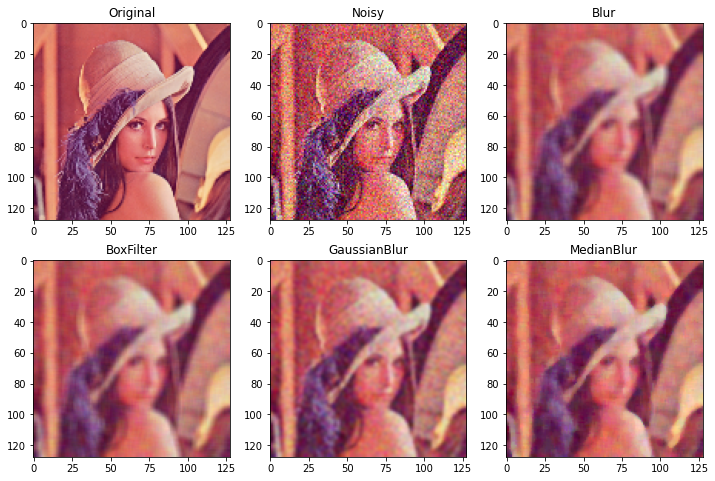
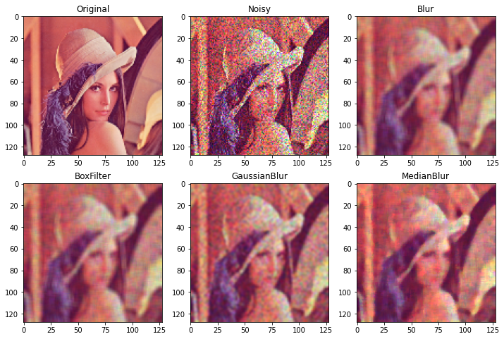
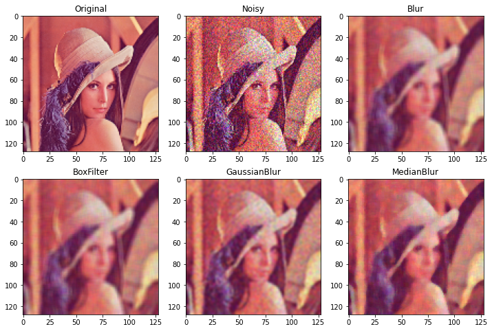
Median filtering is a nonlinear signal processing method that can overcome the blurring of image details caused by linear filters
Blur filtering is effective for images containing Gaussian noise, while median filtering is better for denoising images containing salt and pepper noise

def image_filter(img_noisy, fil_type):
    dict_fil = {1: "Blur", 2: "BoxFilter", 3: "GaussianBlur", 4: "MedianBlur"}
    if fil_type >= 1 and fil_type <= 4:
        print("Type ->", dict_fil[fil_type])
    else:
        print("Error: invalid dict_fil!")
        return None
    return {
        1: cv2.blur(img_noisy, ksize=(5, 5), borderType=cv2.BORDER_DEFAULT),
        2: cv2.boxFilter(img_noisy, ddepth=-1, ksize=(5, 5), 
                         borderType=cv2.BORDER_DEFAULT),
        3: cv2.GaussianBlur(img_noisy, ksize=(5, 5), sigmaX=0, sigmaY=0,
                            borderType=cv2.BORDER_DEFAULT),
        4: cv2.medianBlur(img_noisy, ksize=5)
    }[fil_type]

def show_filter(img_rgb, img_noise):
    img_filter = [image_filter(img_noise, i + 1) for i in range(4)]
    titles = ["Original", "Noisy", "Blur", "BoxFilter", "GaussianBlur", "MedianBlur"]
    img_filter.insert(0, img_noise)
    img_filter.insert(0, img_rgb)
    plt.figure(figsize=(12, 8))
    for i in range(6):
        plt.subplot(2, 3, 1 + i)
        plt.imshow(img_filter[i], norm=no_norm)
        plt.title(titles[i])

show_filter(img_rgb, img_noisy_four[0])

Type -> Blur
Type -> BoxFilter
Type -> GaussianBlur
Type -> MedianBlur

png

show_filter(img_rgb, img_noisy_four[1])

Type -> Blur
Type -> BoxFilter
Type -> GaussianBlur
Type -> MedianBlur

png

show_filter(img_rgb, img_noisy_four[2])

Type -> Blur
Type -> BoxFilter
Type -> GaussianBlur
Type -> MedianBlur

png

show_filter(img_rgb, img_noisy_four[3])

Type -> Blur
Type -> BoxFilter
Type -> GaussianBlur
Type -> MedianBlur

png

Auto-encoder

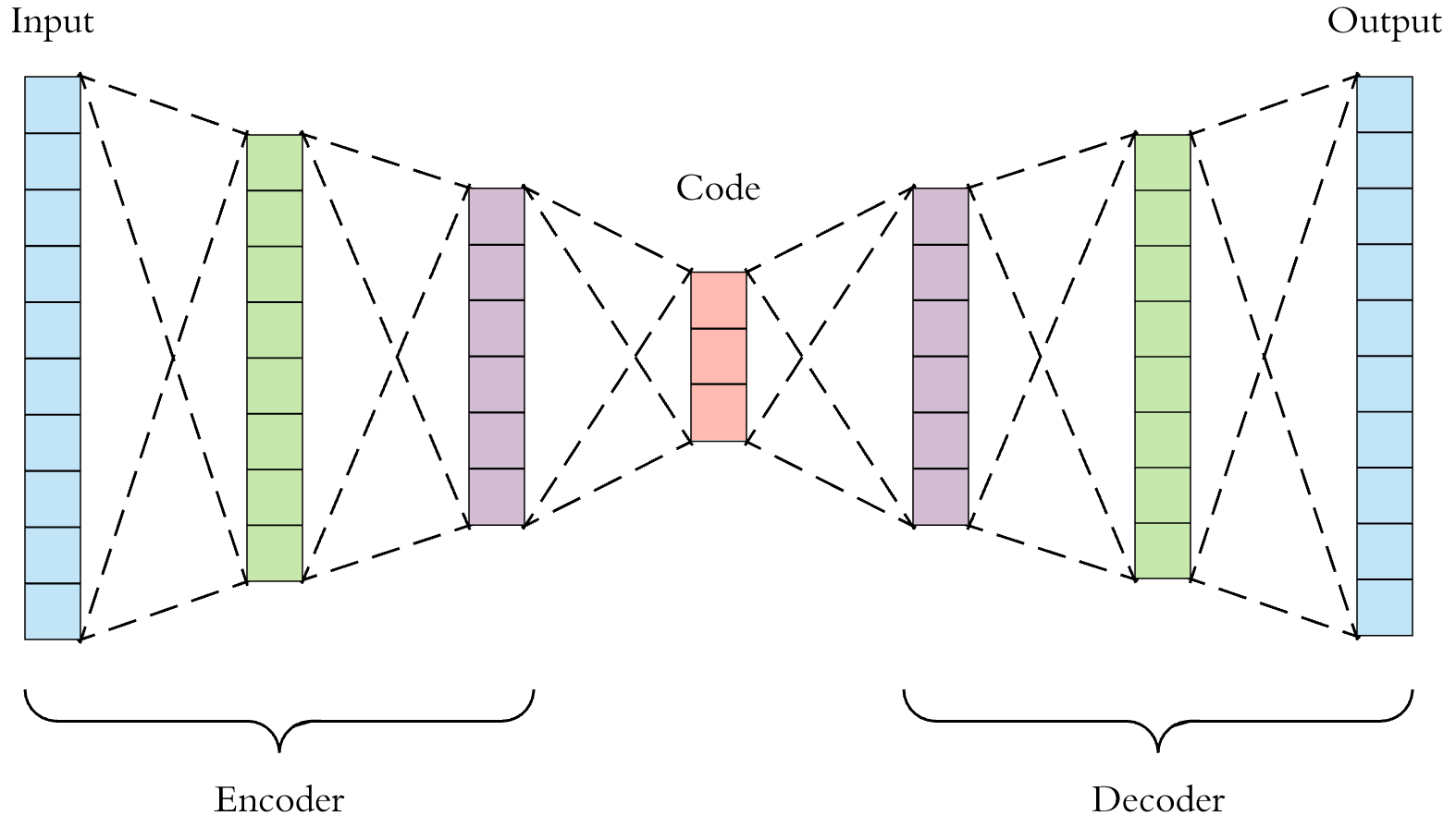
An autoencoder is a type of artificial neural network used to learn efficient codings of unlabeled data (unsupervised learning)
The encoding is validated and refined by attempting to regenerate the input from the encoding
The autoencoder learns a representation (encoding) for a set of data, typically for dimensionality reduction, by training the network to ignore insignificant data (noise)

Regularized autoencoders

Sparse autoencoder (SAE)
- Learning representations in a way that encourages sparsity improves performance on classification tasks
- Sparse autoencoders may include more (rather than fewer) hidden units than inputs, but only a small number of the hidden units are allowed to be active at the same time (thus, sparse)
- This constraint forces the model to respond to the unique statistical features of the training data
Contractive autoencoder (CAE)
- A contractive autoencoder adds an explicit regularizer in its objective function that forces the model to learn an encoding robust to slight variations of input values
- This regularizer corresponds to the Frobenius norm of the Jacobian matrix of the encoder activations with respect to the input
- Since the penalty is applied to training examples only, this term forces the model to learn useful information about the training distribution
Denoising autoencoder (DAE)
- Denoising autoencoders (DAE) try to achieve a good representation by changing the reconstruction criterion
- Indeed, DAEs take a partially corrupted input and are trained to recover the original undistorted input. In practice, the objective of denoising autoencoders is that of cleaning the corrupted input, or denoising. Two assumptions are inherent to this approach
  - Higher level representations are relatively stable and robust to the corruption of the input
  - To perform denoising well, the model needs to extract features that capture useful structure in the input distribution
- In other words, denoising is advocated as a training criterion for learning to extract useful features that will constitute better higher level representations of the input
The training process of a DAE works as follows
- The initial input \({\displaystyle x}x\) is corrupted into \({\displaystyle {\boldsymbol {\tilde {x}}}}\) through stochastic mapping \({\displaystyle {\boldsymbol {\tilde {x}}}\thicksim q_{D}({\boldsymbol {\tilde {x}}} \vert {\boldsymbol {x}})}\)
- The corrupted input \({\displaystyle {\boldsymbol {\tilde {x}}}}\) is then mapped to a hidden representation with the same process of the standard autoencoder, \({\displaystyle {\boldsymbol {h}}=f_{\theta }({\boldsymbol {\tilde {x}}})=s({\boldsymbol {W}}{\boldsymbol {\tilde {x}}}+{\boldsymbol {b}})}\)
- From the hidden representation the model reconstructs \({\displaystyle {\boldsymbol {z}}=g_{\theta '}({\boldsymbol {h}})}\)
The model’s parameters \({\displaystyle \theta }\) and \({\displaystyle \theta '}\) are trained to minimize the average reconstruction error over the training data, specifically, minimizing the difference between \({\displaystyle }{\displaystyle {\boldsymbol {z}}}\) and the original uncorrupted input \({\displaystyle {\boldsymbol {x}}}{}\)
Note that each time a random example \({\displaystyle {\boldsymbol {x}}}{\boldsymbol {}}\) is presented to the model, a new corrupted version is generated stochastically on the basis of \({\displaystyle q_{D}({\boldsymbol {\tilde {x}}}\vert{\boldsymbol {x}})}\)
The above-mentioned training process could be applied with any kind of corruption process. Some examples might be additive isotropic Gaussian noise, masking noise or salt-and-pepper noise
The corruption of the input is performed only during training
After training, no corruption is added

Concrete autoencoder

The concrete autoencoder is designed for discrete feature selection
A concrete autoencoder forces the latent space to consist only of a user-specified number of features
The concrete autoencoder uses a continuous relaxation of the categorical distribution to allow gradients to pass through the feature selector layer, which makes it possible to use standard backpropagation to learn an optimal subset of input features that minimize reconstruction loss.

Variational autoencoder (VAE)

Despite the architectural similarities with basic autoencoders, VAEs are architecture with different goals and with a completely different mathematical formulation
The latent space is in this case composed by a mixture of distributions instead of a fixed vector
Given an input dataset \({\displaystyle \mathbf {} }\mathbf {x}\) characterized by an unknown probability function \({\displaystyle P({\mathbf {x}})}\) and a multivariate latent encoding vector \({\displaystyle \mathbf {} }\mathbf {z}\) , the objective is to model the data as a distribution \({\displaystyle p_{\theta }(\mathbf {x} )}\), with \({\displaystyle \theta }\) defined as the set of the network parameters so that

\[{\displaystyle p_{\theta }(\mathbf {x} )=\int _{\mathbf {z} }p_{\theta }(\mathbf {x,z} )d\mathbf {z} }\]

from keras.datasets import mnist
from tqdm import tqdm
from torchvision import transforms
import torch.nn as nn
from torch.utils.data import DataLoader, Dataset
import torch
import torch.optim as optim
from torch.autograd import Variable

device = "cuda" if torch.cuda.is_available() else "cpu"

#Here we load the dataset from keras
(x_train, y_train), (x_test, y_test) = mnist.load_data()
print("number of training datapoints ->", len(x_train))
print("number of test datapoints     ->", len(x_test))

number of training datapoints -> 60000
number of test datapoints     -> 10000

plt.figure(figsize=(12, 3))
for i in range(2):
    plt.subplot(1, 4, i + 1)
    plt.imshow(x_train[i * 9], "gray", norm=no_norm)
    plt.title("label: " + str(y_train[i * 9]))
for i in range(2):
    plt.subplot(1, 4, i + 1 + 2)
    plt.imshow(x_test[i * 9], "gray", norm=no_norm)
    plt.title("label: " + str(y_test[i * 9]))

png

def add_noise(img, noise_type="gaussian"):
    row, col = 28, 28
    img = img.astype(np.float32)
    if noise_type == "gaussian":
        return gaussian_noise(img, 42, gray=True)
    elif noise_type == "speckle":
        return speckle(img, 0.42, gray=True)
    else:
        print("Error: Invalid noise_type!")

def data_noise_process_train(data, info):
    noise_types = ["gaussian", "speckle"]
    noise_count = 0
    noise_index = 0
    noise_data = np.zeros(data.shape)

    for i in tqdm(range(len(data))):
        if noise_count < (len(data)/2):
            noise_count += 1
            noise_data[i] = add_noise(data[i], noise_type = noise_types[noise_index])
        else:
            print(noise_types[noise_index], "noise addition completed to images", info)
            noise_index += 1
            noise_count = 0

    print(noise_types[noise_index], " noise addition completed to images", info) 
    return noise_data

x_n_train = data_noise_process_train(x_train, "<X_TRAIN>")
x_n_test = data_noise_process_train(x_test, "<X_TEST>")
y_n_train, y_n_test = y_train, y_test

 53%|███████████████▌             | 32076/60000 [00:04<00:02, 10986.65it/s]

gaussian noise addition completed to images <X_TRAIN>

100%|██████████████████████████████| 60000/60000 [00:07<00:00, 8068.33it/s]

speckle  noise addition completed to images <X_TRAIN>

 66%|███████████████████▊          | 6603/10000 [00:00<00:00, 10562.52it/s]

gaussian noise addition completed to images <X_TEST>

100%|█████████████████████████████| 10000/10000 [00:00<00:00, 10700.87it/s]

speckle  noise addition completed to images <X_TEST>

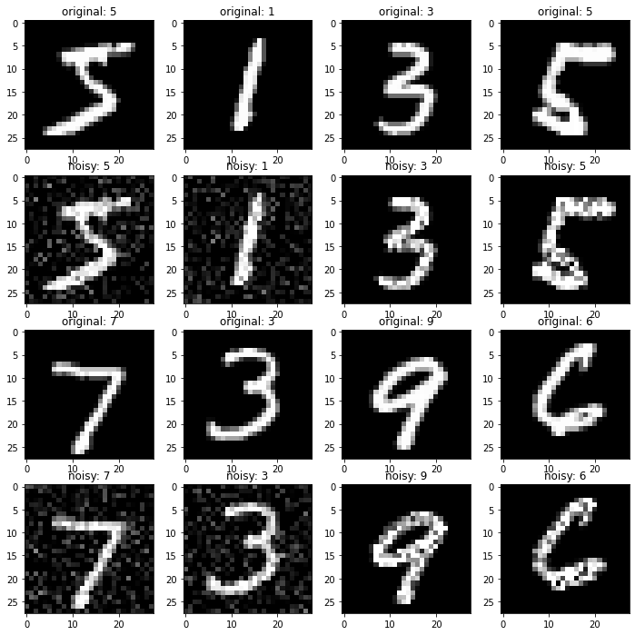
def show_noisy_data(x_train, x_n_train, y_train, x_test, x_n_test, y_test):
    plt.figure(figsize=(12, 12))
    for i in range(4):
        plt.subplot(4, 4, i + 1)
        plt.imshow(x_train[i * 15001], "gray", norm=no_norm)
        plt.title("original: " + str(y_train[i * 15001]))
    for i in range(4):
        plt.subplot(4, 4, i + 1 + 4)
        plt.imshow(x_n_train[i * 15001], "gray", norm=no_norm)
        plt.title("noisy: " + str(y_n_train[i * 15001]))
    for i in range(4):
        plt.subplot(4, 4, i + 1 + 8)
        plt.imshow(x_test[i * 2501], "gray", norm=no_norm)
        plt.title("original: " + str(y_test[i * 2501]))
    for i in range(4):
        plt.subplot(4, 4, i + 1 + 12)
        plt.imshow(x_n_test[i * 2501], "gray", norm=no_norm)
        plt.title("noisy: " + str(y_n_test[i * 2501]))

show_noisy_data(x_train, x_n_train, y_train, x_test, x_n_test, y_test)

png

class noised_dataset(Dataset):
  
    def __init__(self, dataset_noisy, dataset_clean, labels, transform):
        self.noise = dataset_noisy
        self.clean = dataset_clean
        self.labels= labels
        self.transform = transform

    def __len__(self):
        return len(self.noise)

    def __getitem__(self, i):
        x_noise = self.noise[i]
        x_clean = self.clean[i]
        y = self.labels[i]
        if self.transform != None:
            x_noise = self.transform(x_noise)
            x_clean = self.transform(x_clean)
        return (x_noise, x_clean, y)

trainset = noised_dataset(x_n_train, x_train, y_train, 
                          transforms.Compose([transforms.ToTensor()]))
testset = noised_dataset(x_n_test, x_test, y_test, 
                         transforms.Compose([transforms.ToTensor()]))
trainloader = DataLoader(trainset, batch_size=32, shuffle=True)
testloader = DataLoader(testset, batch_size=1, shuffle=True)

class dae_model(nn.Module):
    def __init__(self):
        super(dae_model, self).__init__()
        self.encoder=nn.Sequential(
            nn.Linear(28 * 28, 256), nn.ReLU(True),
            nn.Linear(256, 128), nn.ReLU(True),
            nn.Linear(128, 128), nn.ReLU(True),
            nn.Linear(128, 64), nn.ReLU(True))
        self.decoder=nn.Sequential(
            nn.Linear(64, 128), nn.ReLU(True),
            nn.Linear(128, 128), nn.ReLU(True),
            nn.Linear(128, 256), nn.ReLU(True),
            nn.Linear(256, 28 * 28), nn.Sigmoid())

    def forward(self,x):
        x = self.encoder(x)
        x = self.decoder(x)
        return x

def train_dae_model(trainloader, epochs=100):
    model = dae_model().to(device)
    criterion = nn.MSELoss()
    optimizer = optim.SGD(model.parameters(), lr=0.0005, weight_decay=1e-5)
    # scheduler = optim.lr_scheduler.ExponentialLR(optimizer, gamma=0.99)
    losslist = list()
    running_loss = 0
    for epoch in range(epochs):
        for dirty,clean,label in tqdm(trainloader):
            dirty = dirty.view(dirty.size(0), -1).type(torch.FloatTensor)
            clean = clean.view(clean.size(0), -1).type(torch.FloatTensor)
            dirty, clean = dirty.to(device), clean.to(device)
            #-----------------Forward Pass----------------------
            output = model(dirty)
            loss = criterion(output, clean)
            #-----------------Backward Pass---------------------
            optimizer.zero_grad()
            loss.backward()
            optimizer.step()
            #-----------------Log-------------------------------
            running_loss += loss.item()
        losslist.append(running_loss/len(trainloader))
        running_loss = 0
        print("=============> Epoch: {}/{}, Loss:{}".format(epoch + 1, epochs, loss.item()))
    return losslist, model

losslist, model = train_dae_model(trainloader, epochs=1700)

100%|█████████████████████████████████| 1875/1875 [00:12<00:00, 145.86it/s]

=============> Epoch: 1/1700, Loss:0.2316233515739441

100%|█████████████████████████████████| 1875/1875 [00:12<00:00, 150.97it/s]

=============> Epoch: 2/1700, Loss:0.23167133331298828

100%|█████████████████████████████████| 1875/1875 [00:12<00:00, 153.26it/s]

=============> Epoch: 3/1700, Loss:0.2308265119791031

100%|█████████████████████████████████| 1875/1875 [00:12<00:00, 146.38it/s]

=============> Epoch: 4/1700, Loss:0.2303747832775116

100%|█████████████████████████████████| 1875/1875 [00:15<00:00, 119.29it/s]

=============> Epoch: 5/1700, Loss:0.2293112426996231

...
...    
...

100%|██████████████████████████████████| 1875/1875 [00:20<00:00, 92.90it/s]

=============> Epoch: 1696/1700, Loss:0.024330606684088707

100%|██████████████████████████████████| 1875/1875 [00:22<00:00, 82.09it/s]

=============> Epoch: 1697/1700, Loss:0.02372368425130844

100%|██████████████████████████████████| 1875/1875 [00:20<00:00, 90.50it/s]

=============> Epoch: 1698/1700, Loss:0.025429846718907356

100%|██████████████████████████████████| 1875/1875 [00:19<00:00, 93.76it/s]

=============> Epoch: 1699/1700, Loss:0.025284478440880775

100%|██████████████████████████████████| 1875/1875 [00:20<00:00, 93.57it/s]

=============> Epoch: 1700/1700, Loss:0.028134075924754143

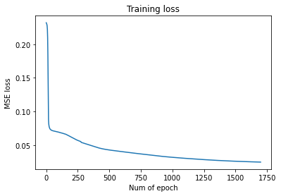
plt.plot(range(len(losslist)), losslist)
plt.title("Training loss")
plt.xlabel("Num of epoch")
plt.ylabel("MSE loss")

Text(0, 0.5, 'MSE loss')

png

def show_preprocess(image):
    image = image.view(1, 28, 28)
    image = image.permute(1, 2, 0).squeeze(2)
    image = image.detach().cpu().numpy()
    return image

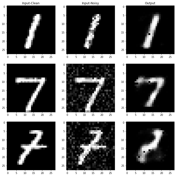
def evaluate_dae(testset):
    f, axes = plt.subplots(3, 3, figsize=(12, 12))
    axes[0, 0].set_title("Input-Clean")
    axes[0, 1].set_title("Input-Noisy")
    axes[0, 2].set_title("Output")
    test_imgs = np.random.randint(0, 10000, size=3)
    for i in range(3):
        dirty = testset[test_imgs[i]][0]
        clean = testset[test_imgs[i]][1]
        label = testset[test_imgs[i]][2]
        dirty = dirty.view(dirty.size(0), -1).type(torch.FloatTensor)
        dirty = dirty.to(device)
        output = model(dirty)

        output = show_preprocess(output)
        dirty = show_preprocess(dirty)

        clean = clean.permute(1, 2, 0).squeeze(2)
        clean = clean.detach().cpu().numpy()

        axes[i, 0].imshow(clean, cmap="gray")
        axes[i, 1].imshow(dirty, cmap="gray")
        axes[i, 2].imshow(output, cmap="gray")

evaluate_dae(testset)

png

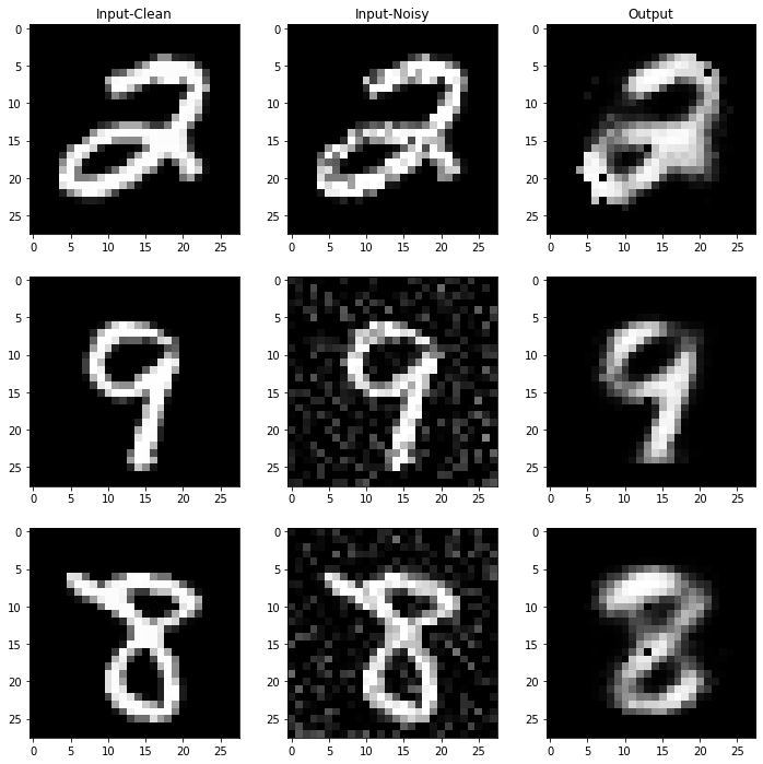
# see another three images and save model
evaluate_dae(testset)
import os
if not os.path.exists("./result"): os.mkdir("./result")
if not os.path.exists("./result/class_2"): os.mkdir("./result/class_2")
torch.save(model.state_dict(), "./result/class_2/dae_mnist.pth")

png

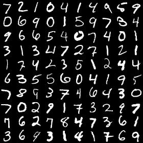
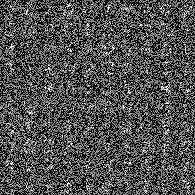
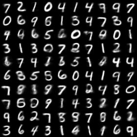
VAE in MNIST

Original input image	Input image with noise	Restored image via VAE

Convolution operation

convolution

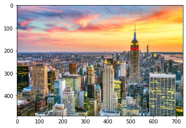
img_bgr = cv2.imread("./images/city.jpg")
img_rgb = cv2.cvtColor(img_bgr, cv2.COLOR_BGR2RGB)
print(img_rgb.shape)
no_norm = mat_color.Normalize(vmin=0, vmax=255, clip=False)
plt.imshow(img_rgb, norm=no_norm)

(489, 730, 3)

<matplotlib.image.AxesImage at 0x1692c93c940>

png

def convolution_single_channel(img, core, core_size):
    height, width = img.shape[0] - core_size, img.shape[1] - core_size
    out = np.zeros(shape=(height, width), dtype=np.int16)
    for i in range(height):
        for j in range(width):
            value = np.sum(core * img[i:i+core_size, j:j+core_size])
            value = value/float(core_size**2.0)
            value = min(value, 255)
            value = max(value, 0)
            out[i][j] = int(value)
    return out

def generate_core(core_size):
    core = np.zeros(shape=(core_size, core_size), dtype=float)
    for i in range(core_size):
        for j in range(core_size):
            core[i][j] = np.random.uniform(-0.5, 2.5)
    return core

def convolution_operation(img, is_random=True, cores=None, core_size=3):
    if is_random:
        cores = [generate_core(core_size) for _ in range(3)]
    if len(img.shape) == 3:
        R, G, B = cv2.split(img)
        R_conv = convolution_single_channel(R, cores[0], core_size)
        G_conv = convolution_single_channel(G, cores[1], core_size)
        B_conv = convolution_single_channel(B, cores[2], core_size)
        return cv2.merge((R_conv, G_conv, B_conv))
    else:
        return convolution_single_channel(img, cores, core_size)

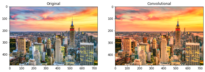
img_con = convolution_operation(img_rgb, is_random=True, core_size=3)
plt.figure(figsize=(12, 4))
plt.subplot(1, 2, 1), print(img_rgb.shape)
plt.imshow(img_rgb, norm=no_norm), plt.title("Original")
plt.subplot(1, 2, 2), print(img_con.shape)
plt.imshow(img_con, norm=no_norm), plt.title("Convolutional")

(489, 730, 3)
(486, 727, 3)

(<matplotlib.image.AxesImage at 0x1692c88ed60>,
 Text(0.5, 1.0, 'Convolutional'))

png

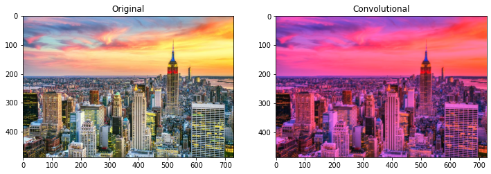
my_cores = [generate_core(3), np.ones((3, 3)) * 0.5, np.ones((3, 3))]
img_con = convolution_operation(img_rgb, is_random=False, cores=my_cores, core_size=3)
plt.figure(figsize=(12, 4))
plt.subplot(1, 2, 1), print(img_rgb.shape)
plt.imshow(img_rgb, norm=no_norm), plt.title("Original")
plt.subplot(1, 2, 2), print(img_con.shape)
plt.imshow(img_con, norm=no_norm), plt.title("Convolutional")

(489, 730, 3)
(486, 727, 3)

(<matplotlib.image.AxesImage at 0x1690a36e070>,
 Text(0.5, 1.0, 'Convolutional'))

png

Pooling operation

pool

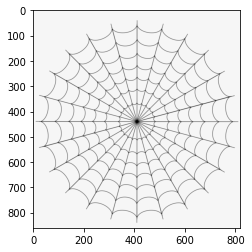
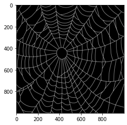
img_light = cv2.imread("./images/spiderweb.png", flags=0)
img_dark = cv2.imread("./images/spiderweb_dark.jpg", flags=0)
print(img_light.shape)
print(img_dark.shape)
no_norm = mat_color.Normalize(vmin=0, vmax=255, clip=False)
plt.imshow(img_light, "gray", norm=no_norm)

(860, 820)
(1000, 1000)

<matplotlib.image.AxesImage at 0x1692d1e8760>

png

plt.imshow(img_dark, "gray", norm=no_norm)

<matplotlib.image.AxesImage at 0x1692d258340>

png

def pool_operation(img, core_size, pool_type=1):
    out = np.zeros((int(img.shape[0]/core_size), int(img.shape[1]/core_size)), dtype=np.int32)
    for i in range(out.shape[0]):
        for j in range(out.shape[1]):
            if pool_type == 1:
                out[i][j] = np.min(img[i*core_size:i*core_size+core_size, 
                                       j*core_size:j*core_size+core_size])
            elif pool_type == 2:
                out[i][j] = np.max(img[i*core_size:i*core_size+core_size, 
                                       j*core_size:j*core_size+core_size])
            elif pool_type == 3:
                out[i][j] = np.mean(img[i*core_size:i*core_size+core_size, 
                                        j*core_size:j*core_size+core_size])
            else:
                 print("Error: Invalid pool_type!")
    print(out.shape)
    return out

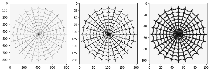
plt.figure(figsize=(12, 4))
plt.subplot(1, 3, 1)
plt.imshow(img_light, "gray", norm=no_norm)
plt.subplot(1, 3, 2)
plt.imshow(pool_operation(img_light, core_size=4), "gray", norm=no_norm)
plt.subplot(1, 3, 3)
plt.imshow(pool_operation(img_light, core_size=8), "gray", norm=no_norm)

(215, 205)
(107, 102)

<matplotlib.image.AxesImage at 0x1692e732970>

png

plt.figure(figsize=(12, 4))
plt.subplot(1, 3, 1)
plt.imshow(img_dark, "gray", norm=no_norm)
plt.subplot(1, 3, 2)
plt.imshow(pool_operation(img_dark, core_size=4, pool_type=2), "gray", norm=no_norm)
plt.subplot(1, 3, 3)
plt.imshow(pool_operation(img_dark, core_size=8, pool_type=2), "gray", norm=no_norm)

(250, 250)
(125, 125)

<matplotlib.image.AxesImage at 0x1692e857eb0>

png

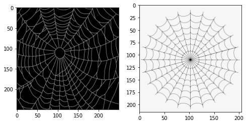
plt.figure(figsize=(8, 4))
plt.subplot(1, 2, 1)
plt.imshow(pool_operation(img_dark, core_size=4, pool_type=3), "gray", norm=no_norm)
plt.subplot(1, 2, 2)
plt.imshow(pool_operation(img_light, core_size=4, pool_type=3), "gray", norm=no_norm)

(250, 250)
(215, 205)

<matplotlib.image.AxesImage at 0x1692cc2b400>

png

The End

2022.3