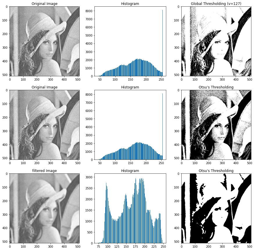
2-1-Basic-Image-Process
Basic image processes
© Haodong Li haodongli@zju.edu.cn
- Grayscale
- Binary-scale
- Otsu’s Binary-scale
Grayscale

- Grayscale conversion algorithms
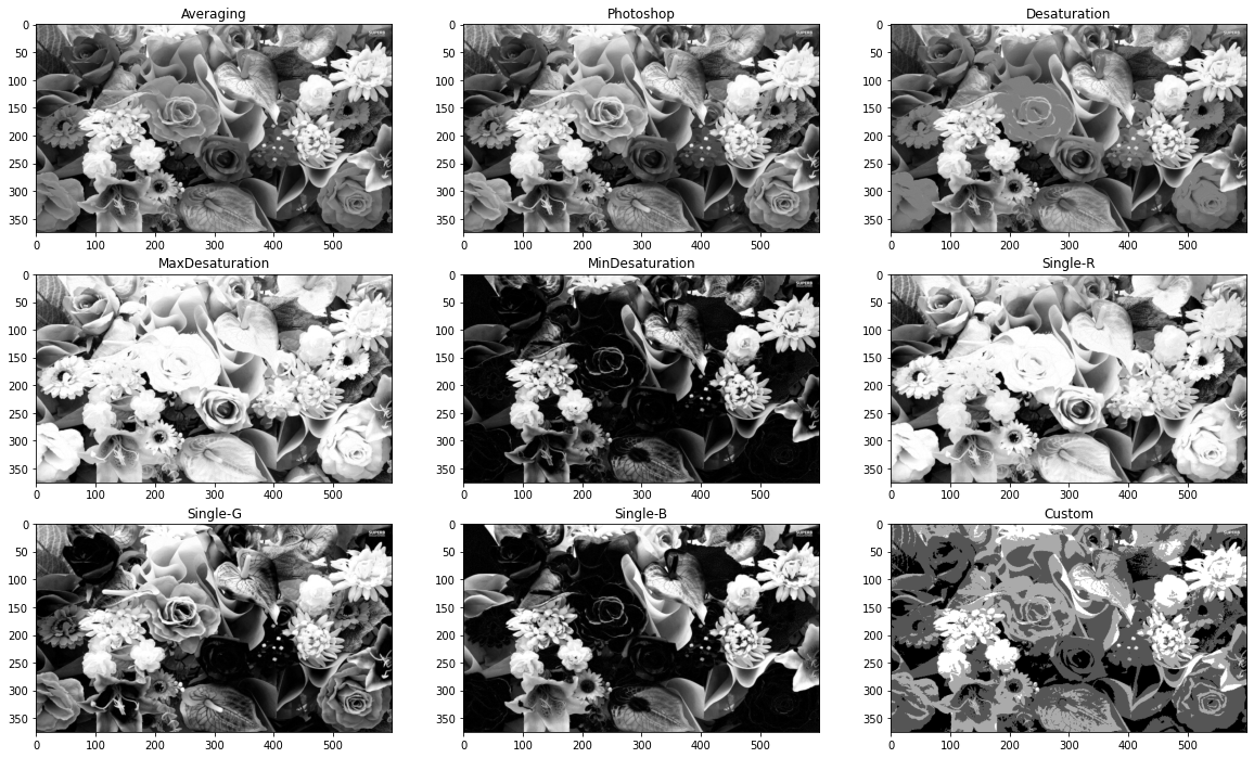
Gray = (Red + Green + Blue) / 3averagingGray = (Red * 0.3 + Green * 0.59 + Blue * 0.11)in Photoshop and GIMPGray = (Red * 0.2126 + Green * 0.7152 + Blue * 0.0722)Gray = (Red * 0.299 + Green * 0.587 + Blue * 0.114)Gray = (Max(Red, Green, Blue) + Min(Red, Green, Blue)) / 2desaturation
- Grayscale conversion algorithms
Gray = Max(Red, Green, Blue)maximum decompositionGray = Min(Red, Green, Blue)minimum decompositionGray = Redsingle color channel (red)Gray = Greensingle color channel (green)Gray = Bluesingle color channel (blue)- Custom algorithms
import cv2
from matplotlib import pyplot as plt
import matplotlib.colors as mat_color

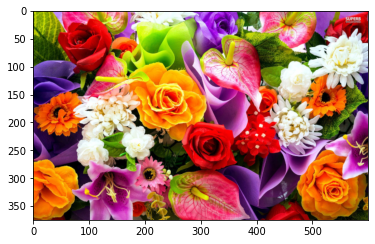
img_bgr = cv2.imread("./images/flowers_small.jpg")
img_rgb = cv2.cvtColor(img_bgr, cv2.COLOR_BGR2RGB)
no_norm = mat_color.Normalize(vmin=0, vmax=255, clip=False)
print(img_rgb.shape)
plt.imshow(img_rgb, norm=no_norm)
(375, 600, 3)


<matplotlib.image.AxesImage at 0x29003c07670>
import numpy as np

def gray_func(pixel, mode=1):
    # default mode is averaging
    if len(pixel) != 3:
        print("Error: invalid pixel shape!")
    # in Python3.10 we have match-case
    # in Python3.9 we not have match-case
    # PyTorch isn't supported in Python3.10
    return {
        1: np.mean(pixel),
        2: np.dot([0.299, 0.587, 0.114], pixel.T),
        3: max(pixel) * 0.5 + min(pixel) * 0.5,
        4: max(pixel),
        5: min(pixel),
        6: pixel[0],
        7: pixel[1],
        8: pixel[2],
    }[mode]
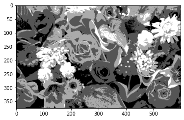
def my_gray_func(pixel):
    number_of_shades = 4
    conversion = 255 / (number_of_shades - 1)
    average = np.mean(pixel)
    return int((average / conversion) + 0.5) * conversion
def grayscale(ori_img, mode=1, show_scale=True):
    if mode < 1 or mode > 9:
        print("Error: invalid mode!")
    height, width, _ = ori_img.shape
    gray_img = np.zeros((height, width), dtype=int)
    for i in range(height):
        for j in range(width):
            if mode == 9:
                gray_img[i][j] = my_gray_func(ori_img[i][j])
            else:
                gray_img[i][j] = gray_func(ori_img[i][j], mode=mode)
    if show_scale:
        print(gray_img.shape)
    return gray_img
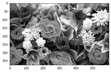
gray_mode_1 = grayscale(img_rgb, mode=1)
plt.imshow(gray_mode_1, 'gray', norm=no_norm)
(375, 600)


<matplotlib.image.AxesImage at 0x29005d0fd60>
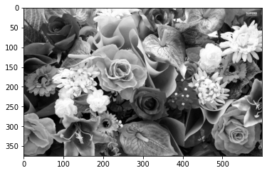
gray_mode_2 = grayscale(img_rgb, mode=2)
plt.imshow(gray_mode_2, 'gray', norm=no_norm)
(375, 600)


<matplotlib.image.AxesImage at 0x29005d89250>
gray_mode_3 = grayscale(img_rgb, mode=3)
plt.imshow(gray_mode_3, 'gray', norm=no_norm)
(375, 600)


<matplotlib.image.AxesImage at 0x29006dc5190>
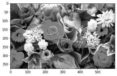
gray_mode_4 = grayscale(img_rgb, mode=4)
plt.imshow(gray_mode_4, 'gray', norm=no_norm)
(375, 600)


<matplotlib.image.AxesImage at 0x29006e24e80>
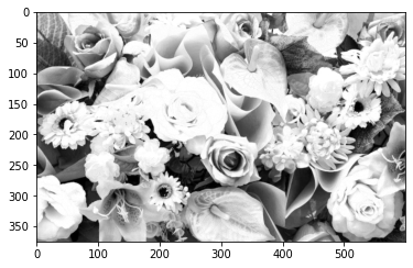
gray_mode_5 = grayscale(img_rgb, mode=5)
plt.imshow(gray_mode_5, 'gray', norm=no_norm)
(375, 600)


<matplotlib.image.AxesImage at 0x29006e8dc70>
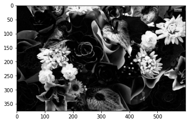
gray_mode_6 = grayscale(img_rgb, mode=6)
plt.imshow(gray_mode_6, 'gray', norm=no_norm)
(375, 600)


<matplotlib.image.AxesImage at 0x29006ef6a00>
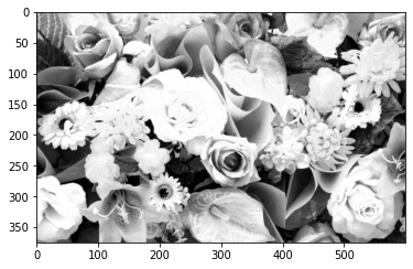
gray_mode_7 = grayscale(img_rgb, mode=7)
plt.imshow(gray_mode_7, 'gray', norm=no_norm)
(375, 600)


<matplotlib.image.AxesImage at 0x29006f63790>
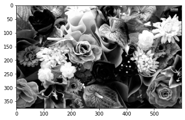
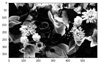
gray_mode_8 = grayscale(img_rgb, mode=8)
plt.imshow(gray_mode_8, 'gray', norm=no_norm)
(375, 600)


<matplotlib.image.AxesImage at 0x29006fd7160>
Custom algorithm
gray_custom = grayscale(img_rgb, mode=9)
plt.imshow(gray_custom, 'gray', norm=no_norm)
(375, 600)


<matplotlib.image.AxesImage at 0x29008004e20>
Show all nine algorithms
titles = ["Averaging", "Photoshop", "Desaturation",
          "MaxDesaturation", "MinDesaturation", "Single-R",
          "Single-G", "Single-B", "Custom"]
images = [gray_mode_1, gray_mode_2, gray_mode_3,
          gray_mode_4, gray_mode_5, gray_mode_6,
          gray_mode_7, gray_mode_8, gray_custom]
plt.figure(figsize = (20, 12))
for i in range(9):
    plt.subplot(3, 3, i + 1)
    plt.imshow(images[i], 'gray', aspect='auto', norm=no_norm)
    plt.title(titles[i])
In OpenCV.cvtColor
gray_img = cv2.cvtColor(img_rgb, cv2.COLOR_RGB2GRAY)
plt.imshow(gray_img, 'gray', norm=no_norm)
<matplotlib.image.AxesImage at 0x290088b0e80>

Binary-scale
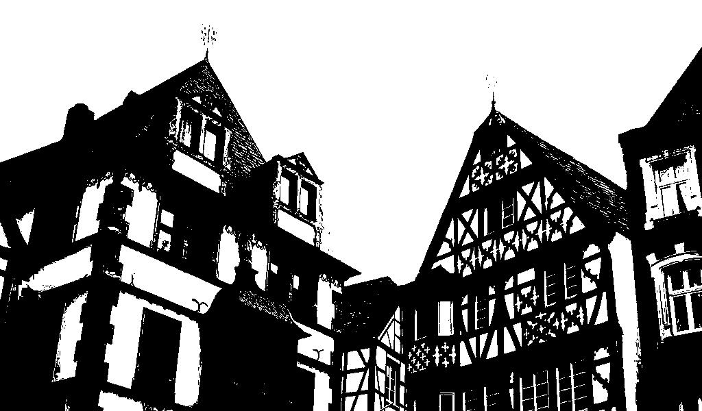
- Set the gray value of each pixel on the image to
0(full black) or255(full white), showing an obvious black and white effect - The commonly used method is: select a certain threshold
T, if the gray value is smaller than the threshold, then0, otherwise255 -
Since that grayscale has been manually implemented at the pixel level before, this time directly using the
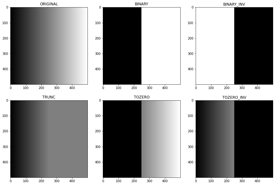
OpenCVlibrary functions cv2.threshold (src, dst, thresh, maxval, type)src: input arraydst: output array (same size and type and same number of channels)thresh: threshold valuemaxval: maximum value to use (cv2.THRESH_BINARYandcv2.THRESH_BINARY_INV)type: thresholding typecv2.THRESH_BINARYcv2.THRESH_BINARY_INVcv2.THRESH_TRUNCcv2.THRESH_TOZEROcv2.THRESH_TOZERO_INVcv2.THRESH_OTSUcv2.THRESH_TRIANGLE
cv2.THRESH_BINARY
cv2.THRESH_BINARY_INV
cv2.THRESH_TRUNC
cv2.THRESH_TOZERO
cv2.THRESH_TOZERO_INV
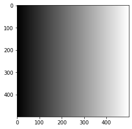
# create a new image for illustrating the concepts
def calculate_value(y):
    return np.array([[((y + 1) * (255 / 500)) for _ in range(500)]]).T

new_img = np.zeros((500, 500))
for i in range(500):
    new_img[:, [i]] = calculate_value(i)
plt.imshow(new_img, 'gray', norm=no_norm)
if cv2.imwrite("./images/gradient.jpg", new_img):
    print("gradient.jpg saved")
gradient.jpg saved
# flag=0 mean read the image in grayscale
ori_img = cv2.imread('./images/gradient.jpg', flags=0)
_, thresh1 = cv2.threshold(ori_img, 127, 255, cv2.THRESH_BINARY)
_, thresh2 = cv2.threshold(ori_img, 127, 255, cv2.THRESH_BINARY_INV)
_, thresh3 = cv2.threshold(ori_img, 127, 255, cv2.THRESH_TRUNC)
_, thresh4 = cv2.threshold(ori_img, 127, 255, cv2.THRESH_TOZERO)
_, thresh5 = cv2.threshold(ori_img, 127, 255, cv2.THRESH_TOZERO_INV)
titles = ['ORIGINAL', 'BINARY','BINARY_INV','TRUNC','TOZERO','TOZERO_INV']
images = [ori_img, thresh1, thresh2, thresh3, thresh4, thresh5]
print("threshold preocess done")
threshold preocess done
plt.figure(figsize = (15, 10))
for i in range(6):
    plt.subplot(2, 3, i + 1)
    plt.imshow(images[i], 'gray', norm=no_norm)
    plt.title(titles[i])
# flag=0 mean read the image in grayscale
ori_img = cv2.imread("./images/flowers_small.jpg", flags=0)
images, titles = [], []
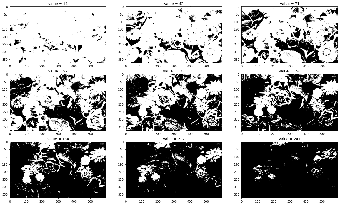
thresholds = [round((i + 0.5) * (255/9.0)) for i in range(9)]
for i in range(9):
    _, thr_img = cv2.threshold(ori_img, thresholds[i], 255, cv2.THRESH_BINARY)
    images.append(thr_img)
    titles.append("value = " + str(thresholds[i]))
print("threshold preocess done")
threshold preocess done
plt.figure(figsize = (20, 12))
for i in range(9):
    plt.subplot(3, 3, i + 1)
    plt.imshow(images[i], 'gray', aspect='auto', norm=no_norm)
    plt.title(titles[i])
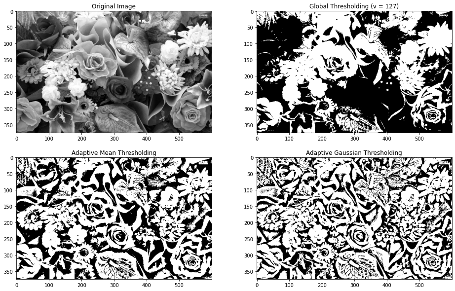
cv2.adaptiveThreshold(src, dst, maxValue, adaptiveMethod, thresholdType, blockSize, C)src: source 8-bit single-channel imagedst: destination image of the same size and the same type as srcmaxValue: non-zero value assigned to the pixels for which the condition is satisfiedadaptiveMethod: adaptive thresholding algorithm to usethresholdType: eithercv2.THRESH_BINARYorcv2.THRESH_BINARY_INVcv2.ADAPTIVE_THRESH_MEAN_Ccv2.ADAPTIVE_THRESH_GAUSSIAN_C
blockSize: size of a pixel neighborhood that is used to calculate a threshold valueC: constant subtracted from the mean or weighted mean
cv2.ADAPTIVE_THRESH_MEAN_C- the threshold value \(T(x, y)\) is a mean of the
blockSize×blockSize(we assumeblockSizeas \(B\) and \(B\in Z\)) neighborhood of \((x, y)\) minus \(C\)
cv2.ADAPTIVE_THRESH_GAUSSIAN_C- the threshold value \(T(x, y)\) is a weighted sum (we assume the weighted matrix is \(W\)) of the \(blockSize×blockSize\) neighborhood of \((x, y)\) minus \(C\)
# flag=0 mean read the image in grayscale
ori_img = cv2.imread("./images/flowers_small.jpg", flags=0)
_, thresh1 = cv2.threshold(ori_img, 127, 255, cv2.THRESH_BINARY)
thresh2 = cv2.adaptiveThreshold(ori_img, 255, cv2.ADAPTIVE_THRESH_MEAN_C,
                                cv2.THRESH_BINARY, 37, 9)
thresh3 = cv2.adaptiveThreshold(ori_img, 255, cv2.ADAPTIVE_THRESH_GAUSSIAN_C,
                                cv2.THRESH_BINARY, 37, 9)
titles = ['Original Image', 'Global Thresholding (v = 127)',
            'Adaptive Mean Thresholding', 'Adaptive Gaussian Thresholding']
images = [ori_img, thresh1, thresh2, thresh3]
print("adaptiveThreshold preocess done")
adaptiveThreshold preocess done
plt.figure(figsize = (16, 10))
for i in range(4):
    plt.subplot(2, 2, i + 1)
    plt.imshow(images[i], 'gray', norm=no_norm)
    plt.title(titles[i])
Otsu’s Binarization
- In global thresholding, we used an arbitrary chosen value as a threshold
- In contrast, Otsu’s method avoids having to choose a value and determines it automatically
- Consider an image with only two distinct image values (bimodal image), where the histogram would only consist of two peaks. A good threshold would be in the middle of those two values. Similarly, Otsu’s method determines an optimal global threshold value from the image histogram
- In order to do so, the
cv2.threshold()function is used, wherecv.THRESH_OTSUis passed as an extra flag. The algorithm then finds the optimal threshold value which is returned as the first output.
# flag=0 mean read the image in grayscale
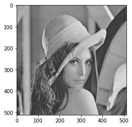
ori_img = cv2.imread("./images/cv.png", flags=0)
plt.imshow(ori_img, 'gray', norm=no_norm)
<matplotlib.image.AxesImage at 0x29008318ca0>
import random

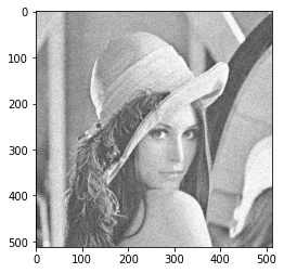
def add_noise(ori_pixel, standard=70):
    return min(ori_pixel + standard - random.uniform(0, standard), 255)

height, width = ori_img.shape
for i in range(height):
    for j in range(width):
        ori_img[i][j] = add_noise(ori_img[i][j])

plt.imshow(ori_img, 'gray', norm=no_norm)
<matplotlib.image.AxesImage at 0x2900884fa30>
# global thresholding
_, th1 = cv2.threshold(ori_img, 127, 255, cv2.THRESH_BINARY)
# Otsu's thresholding
_, th2 = cv2.threshold(ori_img, 0, 255, cv2.THRESH_BINARY + cv2.THRESH_OTSU)
# Otsu's thresholding after Gaussian filtering
blur = cv2.GaussianBlur(ori_img, (15, 15), 0)
_, th3 = cv2.threshold(blur, 0, 255, cv2.THRESH_BINARY + cv2.THRESH_OTSU)
# plot all the images and their histograms
images = [ori_img, 0, th1,
          ori_img, 0, th2,
          blur, 0, th3]
titles = ["Original Image", "Histogram", "Global Thresholding (v=127)",
          "Original Image", "Histogram", "Otsu's Thresholding",
          "filtered Image", "Histogram", "Otsu's Thresholding"]
print("Otsu's threshold preocess done")
Otsu's threshold preocess done
plt.figure(figsize = (15, 15))
for i in range(3):
    plt.subplot(3,3,i*3+1), plt.imshow(images[i*3],"gray",norm=no_norm), plt.title(titles[i*3])
    plt.subplot(3,3,i*3+2), plt.hist(images[i*3].ravel(),256), plt.title(titles[i*3+1])
    plt.subplot(3,3,i*3+3), plt.imshow(images[i*3+2],"gray",norm=no_norm), plt.title(titles[i*3+2])
