Advanced image processes

Perspective transformation
Basic morphological operations

Perspective transformation

Perspective transformation is to project the image onto a new viewing plane

perspective_transformation

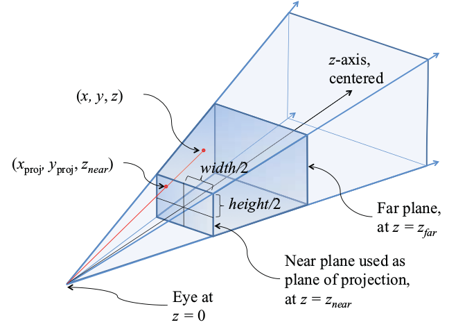
Basic principle of perspective transformation

The general transformation formula is

\[\left[\begin{array}{lll} x^{\prime} & y^{\prime} & w^{\prime} \end{array}\right]=\left[\begin{array}{lll} u & v & w \end{array}\right] \cdot\left[\begin{array}{lll} a_{11} & a_{12} & a_{13} \\ a_{21} & a_{22} & a_{23} \\ a_{31} & a_{32} & a_{33} \end{array}\right] \quad T=\left[\begin{array}{lll} a_{11} & a_{12} & a_{13} \\ a_{21} & a_{22} & a_{23} \\ a_{31} & a_{32} & a_{33} \end{array}\right]=\left[\begin{array}{ll} T_{1} & T_{2} \\ T_{3} & a_{33} \end{array}\right]\]

\(u\), \(v\) are the original pixel coordinates, \(x'\), \(y'\) are the transformed pixel coordinates, \(T\) is the perspective transformation matrix
\(T_1\) represents image linear transformation, \(T_2\) is used to generate image perspective transformation, \(T_3\) represents image translation, \(a_{33}\) is usually taken as \(1\)
Its mathematical expression is as follows

\[x=\frac{x^{\prime}}{w^{\prime}}=\frac{a_{11} u+a_{21} v+a_{31}}{a_{13} u+a_{23} v+a_{33}} \quad y=\frac{y^{\prime}}{w^{\prime}}=\frac{a_{12} u+a_{22} v+a_{32}}{a_{13} u+a_{23} v+a_{33}}\]

Given the four pairs of pixel coordinates of the perspective transformation, the perspective transformation matrix can be obtained
Given a perspective transformation matrix, the perspective transformation can be done
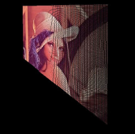
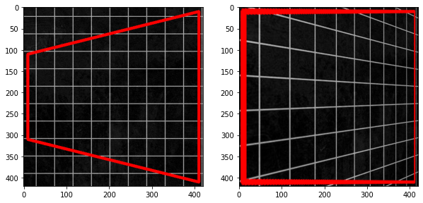
During the perspective transformation process, the area of the original image may become larger, which will cause some pixels of the transformed image to not correspond to the original image, and the background color will appear
Therefore, after the perspective transformation, the transformation map needs to be interpolated to obtain the final target image

Original	No-interpolation	Interpolation

Affine (parallel) transformation

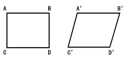
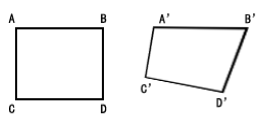
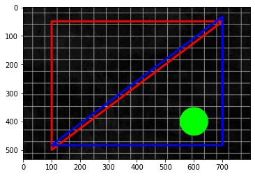
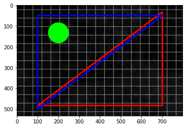
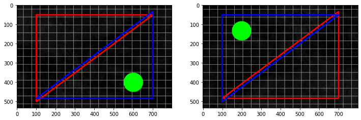
Affine transformation is a special form of perspective transformation, which can maintain the straightness and parallelism of two-dimensional images, and can be used for rotation, translation, scaling, staggering and inversion
Its transformation formula and transformation matrix are as follows

\[\left[\begin{array}{lll} x & y & 1 \end{array}\right]=\left[\begin{array}{lll} x & y^{\prime} & 1 \end{array}\right]=\left[\begin{array}{lll} u & v & 1 \end{array}\right] \cdot\left[\begin{array}{lll} a_{11} & a_{12} & 0 \\ a_{21} & a_{22} & 0 \\ a_{31} & a_{32} & 1 \end{array}\right] \quad T=\left[\begin{array}{lll} a_{11} & a_{12} & 0 \\ a_{21} & a_{22} & 0 \\ a_{31} & a_{32} & 1 \end{array}\right]=\left[\begin{array}{cc} T_{1} & T_{2} \\ T_{3} & 1 \end{array}\right]\]

Affine	Normal

import cv2
from matplotlib import pyplot as plt
import numpy as np
import matplotlib.colors as mat_color

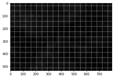
img_ori = cv2.imread("./images/grid.jpg")
print(img_ori.shape)
no_norm = mat_color.Normalize(vmin=0, vmax=255, clip=False)
plt.imshow(img_ori, "gray", norm=no_norm)
# !jt -f office -tf robotosans -tfs 14 -nf robotosans -nfs 14 -t oceans16

(533, 800, 3)

<matplotlib.image.AxesImage at 0x237bde7b670>

png

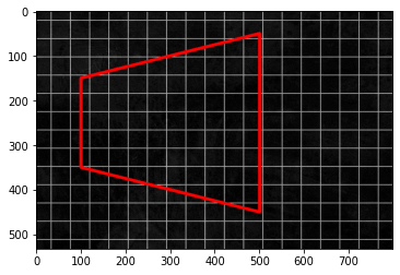
pts = np.array([[100, 150], [500, 50], [500, 450], [100, 350]], np.int32)
pts = pts.reshape((-1, 1, 2))
cv2.polylines(img_ori, [pts], True, (255, 0, 0), thickness=5)
plt.imshow(img_ori, norm=no_norm)

<matplotlib.image.AxesImage at 0x237c0211fd0>

png

# specify input and output coordinates
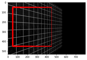
input_pts = np.float32([[100, 150], [500, 50], [500, 450], [100, 350]])
output_pts = np.float32([[50, 50], [450, 50], [450, 450], [50, 450]])
# compute the perspective transform M
M = cv2.getPerspectiveTransform(input_pts, output_pts)
# apply the perspective transformation to the image
img_per = cv2.warpPerspective(img_ori, M,(img_ori.shape[1], img_ori.shape[0]),
                              flags=cv2.INTER_LINEAR)
plt.imshow(img_per, norm=no_norm)

<matplotlib.image.AxesImage at 0x237c0504ca0>

png

plt.figure(figsize=(10, 5))
plt.subplot(1, 2, 1)
plt.imshow(img_ori[50 - 10:450 + 10, 100 - 10:500 + 10], "gray", norm=no_norm)
plt.subplot(1, 2, 2)
plt.imshow(img_per[50 - 10:450 + 10, 50 - 10:450 + 10], norm=no_norm)

<matplotlib.image.AxesImage at 0x237c06c3d90>

png

img_ori = cv2.imread("./images/grid.jpg")
# define the 3 pairs of corresponding points 
start_pts = [[100, 50], [700, 50], [100, 500]]
dst_pts = [[img_ori.shape[1] - 100, img_ori.shape[0] - 50], 
           [img_ori.shape[1] - 700, img_ori.shape[0] - 50], 
           [img_ori.shape[1] - 100, img_ori.shape[0] - 500]]
pts = np.array(start_pts, np.int32)
pts_dst = np.array(dst_pts, np.int32)
pts, pts_dst = pts.reshape((-1, 1, 2)), pts_dst.reshape((-1, 1, 2))
cv2.polylines(img_ori, [pts], True, (255, 0, 0), thickness=5)
cv2.polylines(img_ori, [pts_dst], True, (0, 0, 255), thickness=5)
cv2.circle(img_ori, (600, 400), 50, (0, 255, 0), -1)
plt.imshow(img_ori, norm=no_norm)

<matplotlib.image.AxesImage at 0x237bdf78d30>

png

src_tri = np.array(start_pts).astype(np.float32)
dst_tri = np.array(dst_pts).astype(np.float32)
# calculate the transformation matrix using cv2.getAffineTransform()
warp_mat = cv2.getAffineTransform(src_tri, dst_tri)
# apply the affine transformation using cv2.warpAffine()
warp_dst = cv2.warpAffine(img_ori, warp_mat, (img_ori.shape[1], img_ori.shape[0]))
plt.imshow(warp_dst, norm=no_norm)

<matplotlib.image.AxesImage at 0x237bdfdf8e0>

png

plt.figure(figsize=(12, 7))
plt.subplot(1, 2, 1)
plt.imshow(img_ori, norm=no_norm)
plt.subplot(1, 2, 2)
plt.imshow(warp_dst, norm=no_norm)

<matplotlib.image.AxesImage at 0x237be048ac0>

png

Basic morphological operations

The basic idea of mathematical morphology is to measure and extract the corresponding shape in the image with structural elements with a certain shape, so as to achieve the purpose of image analysis and recognition
It can simplify image data, keep their basic shape properties, and remove irrelevant structures
Mathematical morphology is composed of a set of morphological algebraic operators, and it has 4 basic operations: Dilation, Erosion, Opening and Closing
Based on these basic operations, various mathematical morphological practical algorithms can be derived and combined, which can be used to analyze and process image shape and structure, including image segmentation, feature extraction, boundary detection, image filtering, image enhancement and restoration, etc

Dilation

This operations consists of convolving an image \(A\) with some kernel \(B\), which can have any shape or size, usually a square or circle
The kernel \(B\) has a defined anchor point, usually being the center of the kernel
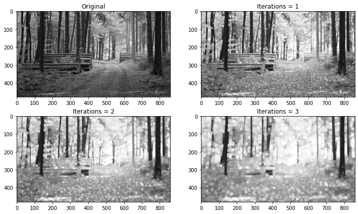
As the kernel \(B\) is scanned over the image, we compute the maximal pixel value overlapped by \(B\) and replace the image pixel in the anchor point position with that maximal value. As you can deduce, this maximizing operation causes bright regions within an image to “grow” (therefore the name dilation)

\[\operatorname{dst}(x, y)=\max _{\left(x^{\prime}, y^{\prime}\right): \text { element }\left(x^{\prime}, y^{\prime}\right) \neq 0} \operatorname{src}\left(x+x^{\prime}, y+y^{\prime}\right)\]

Erosion

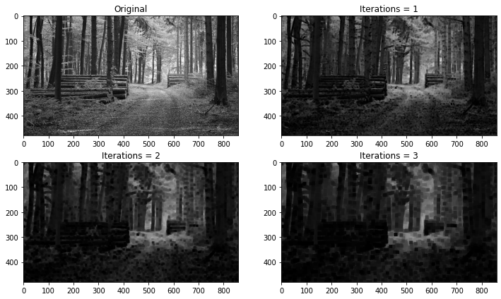
This operation is the sister of dilation. It computes a local minimum over the area of given kernel
As the kernel \(B\) is scanned over the image, we compute the minimal pixel value overlapped by \(B\) and replace the image pixel under the anchor point with that minimal value

\[\operatorname{dst}(x, y)=\min _{\left(x^{\prime}, y^{\prime}\right): \text { element }\left(x^{\prime}, y^{\prime}\right) \neq 0} \operatorname{src}\left(x+x^{\prime}, y+y^{\prime}\right)\]

Opening

Corroded and then expanded

Closing

Expands and then corrodes

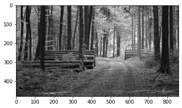
img_ori = cv2.imread("./images/forest.jpg", flags=0)
print(img_ori.shape)
plt.imshow(img_ori, "gray", norm=no_norm)

(480, 860)

<matplotlib.image.AxesImage at 0x237c08f64f0>

png

def show_dilate(img, process_type=1):
    kernel = np.ones((5,5), np.uint8)
    plt.figure(figsize=(12, 7))
    plt.subplot(2, 2, 1)
    plt.imshow(img, "gray", norm=no_norm), plt.title("Original")
    for i in range(3):
        plt.subplot(2, 2, 2 + i)
        if process_type == 1:
            plt.imshow(cv2.dilate(img, kernel, iterations=i+1), "gray", norm=no_norm)
        elif process_type == 2:
            plt.imshow(cv2.erode(img, kernel, iterations=i+1), "gray", norm=no_norm)
        else:
            print("Error: Invalid process_type!")
        plt.title("Iterations = " + str(i+1))

show_dilate(img_ori, process_type=1)

png

show_dilate(img_ori, process_type=2)

png

def show_morphology_specific(img, type_process=1):
    kernel = np.ones((5, 5), np.uint8)
    plt.figure(figsize=(12, 4))
    plt.subplot(1, 2, 1)
    plt.imshow(img, "gray", norm=no_norm), plt.title("ORIGINAL")
    op_s = [cv2.MORPH_OPEN, cv2.MORPH_CLOSE, cv2.MORPH_GRADIENT, 
            cv2.MORPH_TOPHAT, cv2.MORPH_BLACKHAT]
    titles = ["OPEN", "CLOSE", "GRADIENT", "TOP-HAT", "BLACK-HAT"]
    plt.subplot(1, 2, 2)
    plt.imshow(cv2.morphologyEx(img, op_s[type_process - 1], kernel), 
               "gray", norm=no_norm)
    plt.title(titles[type_process - 1])

show_morphology_specific(img_ori, type_process=1)

png

show_morphology_specific(img_ori, type_process=2)

png

show_morphology_specific(img_ori, type_process=3)

png

show_morphology_specific(img_ori, type_process=4)

png

show_morphology_specific(img_ori, type_process=5)

png

def show_morphology(img):
    kernel = np.ones((5, 5), np.uint8)
    plt.figure(figsize=(21, 8))
    plt.subplot(2, 3, 1)
    plt.imshow(img, "gray", norm=no_norm), plt.title("ORIGINAL")
    op_s = [cv2.MORPH_OPEN, cv2.MORPH_CLOSE, cv2.MORPH_GRADIENT, 
            cv2.MORPH_TOPHAT, cv2.MORPH_BLACKHAT]
    titles = ["OPEN", "CLOSE", "GRADIENT", "TOP-HAT", "BLACK-HAT"]
    for i in range(5):
        plt.subplot(2, 3, i + 2)
        plt.imshow(cv2.morphologyEx(img, op_s[i], kernel), "gray", norm=no_norm)
        plt.title(titles[i])

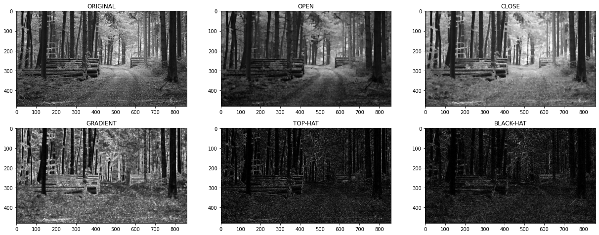
show_morphology(img_ori)